Caution

Under construction…beep beep beep…

Energetic constraints

Energetic constraints

One of the benefits of working with a Hamiltonian is insight into the dynamics can be immediately attained with some careful attention.

Recall from the theory of Hamiltonian systems that any Hamiltonian explicitly independent of time is a constant of motion. This means that our Hamiltonian will:

1. Be a conserved quantity along any solution trajectory

2. Give insight into how the variables are dynamically constrained together

We’re going to explore these ideas a little bit to see what we can understand about the dynamics before writing the equations of motion.

Permissible Motion

Recall the Hamiltonian and the relations between the momenta and the rotating position/velocity variables.

\[\begin{split}H &= \frac{1}{2}\Big((p_x + y)^2 + (p_y - x)^2 + p_z^2\Big) + \bar{U}(x,y,z) \\ \dot{x} & = p_x + y \\ \dot{y} & = p_y - x \\ \dot{z} & = p_z\end{split}\]

It’s clear then that

\[H = \frac{1}{2}\Big(\underbrace{(p_x + y)^2 + (p_y - x)^2 + p_z^2}_{\dot{x}^2 + \dot{y}^2 + \dot{z}^2}\Big) + \bar{U}(x,y,z),\]

where \(H\) is constant along trajectories. A natural case to consider from here is to ask what happens when \(\dot{x}=\dot{y}=\dot{z}=0\).

• This means the Hamiltonian’s value is set purely by position for all trajectories having any instance in which \(\dot{x}=\dot{y}=\dot{z}=0\)

In this case, the Hamiltonian reduces to \(H = \bar{U}\), or rather

\[\bar{U}(x,y,z) = \mathrm{constant}.\]

We have exactly what defines an implicit surface in three dimensions! By fixing \(\mu\), we can see what the energy surface looks like for all trajectories having \(\dot{x} = \dot{y} = \dot{z} = 0\) across all values of the Hamiltonian.

Zero Velocity Curves

To better understand the realms of permissible motion, let’s first also consider the case when \(z = 0\). Having both \(z=\dot{z}=0\) means that the motion is entirely planar such that all motion is happening in the \((x,y)\) plane. The pseudopotential correspondingly becomes

\[\bar{U}(x,y,0) = \mathrm{constant},\]

where the constant is the value of the Hamiltonian \(H(x,y,0,0,0,0)\).

Aside

Before talking about the constant, it’ll first be helpful to know what \(\bar{U}(x,y,0)\) looks like in the sense of a normal bivariate function.

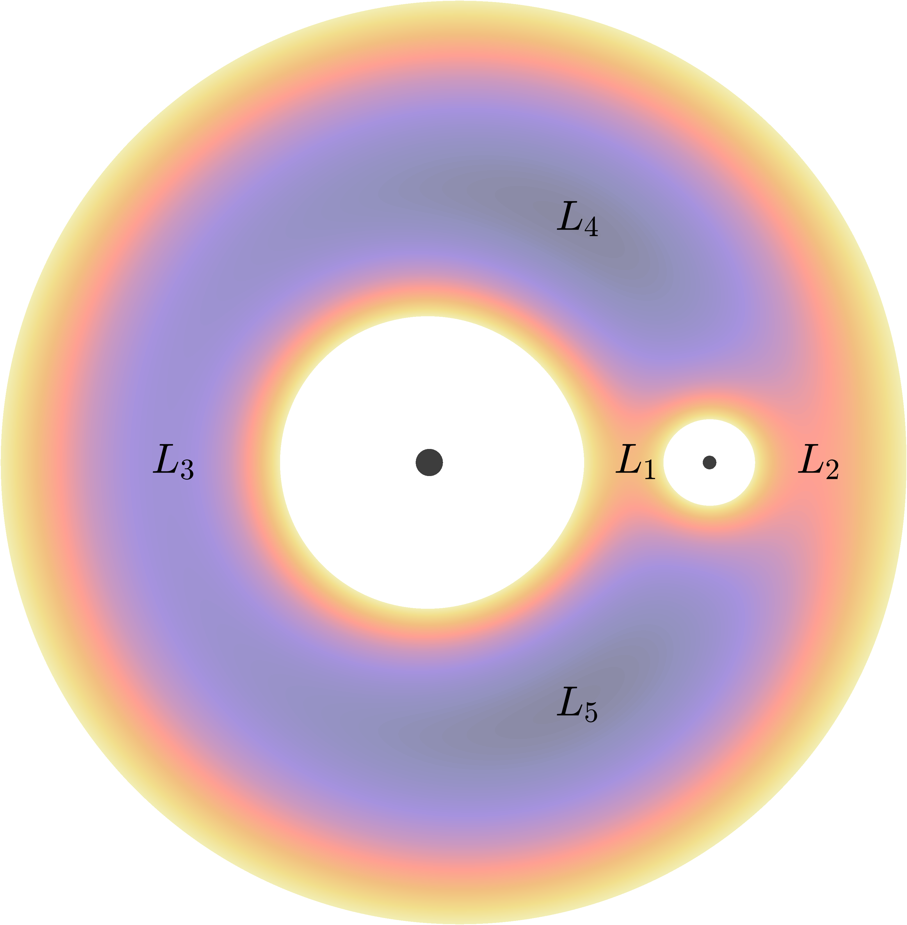
Fig. 8 The pseudopotential shown as a height function for \(\mu = 0.1\).

The five points labelled \(L_1\) through \(L_5\) mark the locations of the pseudopotential’s local extrema (known as the Lagrange points, or libration points)

We have an implicit function of two variables that describes the boundary at which trajectories have \(z = \dot{x} = \dot{y} = \dot{z} = 0\) at a fixed \(\mu\) and Hamiltonian energy. In other words, the boundaries of permissible planar motion at a fixed Hamiltonian energy are given by the level sets of the pseudopotential. These level sets are called the zero velocity curves (due to the condition \(\dot{x} = \dot{y} = \dot{z} = 0\)), which are also sometimes called the Hill curves.

Fig. 9 Level sets of \(\bar{U}(x,y,0) = H\), which define the boundaries of permissible motion at each individual Hamiltonian energy, for \(\mu = 0.1\)

The colored region is called the forbidden realm because it is energetically forbidden for an initial condition at the corresponding Hamiltonian value to be placed there. Correspondingly, the trajectory associated with this same initial condition can also never enter the forbidden realm.

Why is this true?

• The velocities appear in the Hamiltonian as a kinetic energy with \(\dot{x}^2+\dot{y}^2+\dot{z}^2 \geq 0\)

• Entering the forbidden realm results in \(\dot{x}^2+\dot{y}^2+\dot{z}^2 < 0\), which is not physically possible

An intuitive takeaway is that higher energies reduce the size of the forbidden realm until, at a critical value, the forbidden realm disappears completely. We will see soon that this critical value is \(H = -1.5\)

Zero Velocity Surface

The idea of the zero velocity curves can be extended to three dimensions by dropping the assumption that \(z = 0\). That is,

\[\bar{U}(x,y,z) = \mathrm{constant},\]

where the constant is the value of the Hamiltonian \(H(x,y,z,0,0,0)\). In effect, the lines that make up the boundary of the zero velocity curves become a surface to form the zero velocity surface, also sometimes called the Hill surface.

Note

The pseudopotential is symmetric in \(y\) and \(z\).

\[\bar{U}(x,y,z) = \bar{U}(x,-y,z) = \bar{U}(x,y,-z) = \bar{U}(x,-y,-z)\]

Because the pseudopotential is symmetric about \(y\), we can visualize the zero velocity surface using a cross-section with the understanding that the other half of the surface is simply mirrored over the \((x,z)\) plane.

Fig. 10 Level sets of \(\bar{U}(x,y,z) = H\), which define the boundaries of permissible motion at each individual Hamiltonian energy, for \(\mu = 0.1\)

The Five Energy Cases

Without loss of generality, we can consider just the two-dimensional zero velocity curves to understand the qualitative changes happening in the pseudopotential’s level sets.

Jacobi’s Constant

---

References

1. Koon, W.S., Lo, M.W., Marsden, J.E., Ross, S.D. (2022) Dynamical Systems, the Three-Body Problem and Space Mission Design. Marsden Books, ISBN 978-0-615-24095-4.