Inertial and rotating coordinates

Inertial and rotating coordinates

Before we write the Hamiltonian for the CRTBP, we have to understand that its expression will depend on

• The frame, and

• The variables in the frame

Being able to interpret the Hamiltonian’s variables correctly, as well as being comfortable performing coordinate transformations to switch into different representations, will have a lot of value in the long run. So with that, let’s dive in!

Position and velocity

The most intuitively understandable set of coordinates in any frame is undoubtedly that of position and velocity. As such, converting position/velocity states between the inertial and rotating frames is fundamentally important.

Subtle assumption

The inertial frame aligns with the rotating frame at \(t=0\).

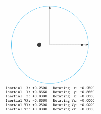
Suppose that the position of a particle is represented in inertial coordinates by \((X,Y,Z)\) and rotating coordinates \((x,y,z)\). The two sets of coordinates are related by

\[\begin{split}\begin{pmatrix}X \\ Y \\ Z\end{pmatrix} = \underbrace{\begin{pmatrix}\cos t & -\sin t & 0 \\ \sin t & \cos t & 0 \\ 0 & 0 & 1\end{pmatrix}}_{\mathbf{R}(t)}\begin{pmatrix}x \\ y \\ z\end{pmatrix}\end{split}\]

Likewise, the inertial velocity \((\dot{X}, \dot{Y}, \dot{Z})\) and rotating velocity \((\dot{x}, \dot{y}, \dot{z})\) are related to each other by simply taking a derivative and applying the chain rule.

\[\begin{split}\begin{pmatrix}\dot{X} \\ \dot{Y} \\ \dot{Z}\end{pmatrix} = \mathbf{R}(t) \begin{pmatrix}\dot{x}-y \\ \dot{y}+x \\ \dot{z}\end{pmatrix}\end{split}\]

Proof

\[\begin{split}\begin{pmatrix}\dot{X} \\ \dot{Y} \\ \dot{Z}\end{pmatrix} &= \frac{d}{dt}\left[\mathbf{R}(t)\begin{pmatrix}x \\ y \\ z\end{pmatrix}\right] \\ &= \dot{\mathbf{R}}(t)\begin{pmatrix}x \\ y \\ z\end{pmatrix} + \mathbf{R}(t)\begin{pmatrix}\dot{x} \\ \dot{y} \\ \dot{z}\end{pmatrix} \\ &= -\mathbf{R}(t)\mathbf{J}\begin{pmatrix}x \\ y \\ z\end{pmatrix} + \mathbf{R}(t)\begin{pmatrix}\dot{x} \\ \dot{y} \\ \dot{z}\end{pmatrix} \\ &= \mathbf{R}(t)\left[-\mathbf{J}\begin{pmatrix}x \\ y \\ z\end{pmatrix} + \begin{pmatrix}\dot{x} \\ \dot{y} \\ \dot{z}\end{pmatrix}\right] \\ &= \mathbf{R}(t) \begin{pmatrix}\dot{x}-y \\ \dot{y}+x \\ \dot{z}\end{pmatrix},\end{split}\]

where \(\mathbf{J}\) is called the symplectic matrix.

\[\begin{split}\mathbf{J} = \begin{pmatrix}0 & 1 & 0 \\ -1 & 0 & 0 \\ 0 & 0 & 0\end{pmatrix}\end{split}\]

Putting both transformations together, we can relate the entire inertial state \((X, Y, Z, \dot{X}, \dot{Y}, \dot{Z})\) with the rotating state \((x, y, z, \dot{x}, \dot{y}, \dot{z})\) by the following state transformation matrix.

\[\begin{split}\begin{pmatrix}X \\ Y \\ Z \\ \dot{X} \\ \dot{Y} \\ \dot{Z}\end{pmatrix} = \underbrace{\begin{pmatrix}\cos t & -\sin t & 0 & 0 & 0 & 0 \\ \sin t & \cos t & 0 & 0 & 0 & 0 \\ 0 & 0 & 1 & 0 & 0 & 0 \\ -\sin t & -\cos t & 0 & \cos t & -\sin t & 0 \\ \cos t & -\sin t & 0 & \sin t & \cos t & 0 \\ 0 & 0 & 0 & 0 & 0 & 1\end{pmatrix}}_{\begin{pmatrix}\mathbf{R}(t) & \mathbf{0} \\ \dot{\mathbf{R}}(t) & \mathbf{R}(t)\end{pmatrix}}\begin{pmatrix}x \\ y \\ z \\ \dot{x} \\ \dot{y} \\ \dot{z}\end{pmatrix}\end{split}\]

The other transformation, to the rotating state from the inertial state, is given similarly.

\[\begin{split}\begin{pmatrix}x \\ y \\ z \\ \dot{x} \\ \dot{y} \\ \dot{z}\end{pmatrix} = \underbrace{\begin{pmatrix}\cos t & \sin t & 0 & 0 & 0 & 0 \\ -\sin t & \cos t & 0 & 0 & 0 & 0 \\ 0 & 0 & 1 & 0 & 0 & 0 \\ -\sin t & \cos t & 0 & \cos t & \sin t & 0 \\ -\cos t & -\sin t & 0 & -\sin t & \cos t & 0 \\ 0 & 0 & 0 & 0 & 0 & 1\end{pmatrix}}_{\begin{pmatrix}\mathbf{R}^T(t) & \mathbf{0} \\ \dot{\mathbf{R}}^T(t) & \mathbf{R}^T(t)\end{pmatrix}}\begin{pmatrix}X \\ Y \\ Z \\ \dot{X} \\ \dot{Y} \\ \dot{Z}\end{pmatrix}\end{split}\]

Fig. 6 Inertial and rotating position/velocity states